1
2
3
4
5
6
7
8
9
10
11
12
13
14
15
16
17
18
19
20
21
22
23
24
25
26
27
28
29
30
31
32
33
34
35
36
37
38
39
40
41
42
43
44
45
46
47
48
49
50
51
52
53
54
55
56
57
58
59
60
61
62
63
64
65
66
67
68
69
70
71
72
73
74
75
76
77
78
79
80
81
82
83
84
85
86
87
88
89
90
91
92
93
94
95
96
97
98
99
100
101
102
103
104
105
106
107
108
109
110
111
112
113
114
115
116
117
118
119
120
121
122
123
124
125
126
127
128
129
130
131
132
133
134
135
136
137
138
139
140
141
142
143
144
145
146
147
148
149
150
151
152
153
154
155
156
157
158
159
160
161
162
163
164
165
| from scipy.linalg import orth
import matplotlib.pyplot as plt
import numpy as np
import torch
import torch.nn as nn
import torch.nn.functional as F
device = torch.device("cuda:0" if torch.cuda.is_available() else "cpu")
class LISTA(nn.Module):
def __init__(self, n, m, W_e, max_iter, L, theta):
"""
n: 输入维度
m: 稀疏表示的维度
W_e: 字典
max_iter: 最大迭代次数
L: Lipschitz常数
theta: 阈值
"""
super(LISTA, self).__init__()
self._W = nn.Linear(in_features=n, out_features=m, bias=False)
self._S = nn.Linear(in_features=m, out_features=m,
bias=False)
self._S2 = nn.Linear(in_features=m, out_features=m,
bias=False)
self._S3 = nn.Linear(in_features=m, out_features=m,
bias=False)
self.shrinkage = nn.Softshrink(theta)
self.theta = theta
self.max_iter = max_iter
self.A = W_e
self.L = L
def weights_init(self):
"""
按照伪代码来初始化S和W_e
"""
A = self.A.cpu().numpy()
L = self.L
S = torch.from_numpy(np.eye(A.shape[1]) - (1/L)*np.matmul(A.T, A))
S = S.float().to(device)
W = torch.from_numpy((1/L)*A.T)
W = W.float().to(device)
self._S.weight = nn.Parameter(S)
self._S2.weight = nn.Parameter(S)
self._S3.weight = nn.Parameter(S)
self._W.weight = nn.Parameter(W)
def forward(self, y):
"""
前向推断步,利用自动求导机制不需要再求解导数
"""
x = self.shrinkage(self._W(y))
if self.max_iter == 1:
return x
for iter in range(self.max_iter):
x = self.shrinkage(self._W(y) + self._S(x))
x = self.shrinkage(self._W(y) + self._S2(x))
x = self.shrinkage(self._W(y) + self._S3(x))
return x
def train_lista(Y, dictionary, a, L, max_iter=30):
"""
由于需要训练权重,所以还需要使用一个包装函数来训练网络
"""
n, m = dictionary.shape
n_samples = Y.shape[0]
batch_size = 32
steps_per_epoch = n_samples // batch_size
Y = torch.from_numpy(Y)
Y = Y.float().to(device)
W_d = torch.from_numpy(dictionary)
W_d = W_d.float().to(device)
net = LISTA(n, m, W_d, max_iter=30, L=L, theta=a/L)
net = net.float().to(device)
net.weights_init()
learning_rate = 1e-2
criterion1 = nn.MSELoss()
criterion2 = nn.L1Loss()
all_zeros = torch.zeros(batch_size, m).to(device)
optimizer = torch.optim.SGD(
net.parameters(), lr=learning_rate, momentum=0.9)
loss_list = []
for epoch in range(100):
index_samples = np.random.choice(
a=n_samples, size=n_samples, replace=False, p=None)
Y_shuffle = Y[index_samples]
for step in range(steps_per_epoch):
Y_batch = Y_shuffle[step*batch_size:(step+1)*batch_size]
optimizer.zero_grad()
X_h = net(Y_batch)
Y_h = torch.mm(X_h, W_d.T)
loss1 = criterion1(Y_batch.float(), Y_h.float())
loss2 = a * criterion2(X_h.float(), all_zeros.float())
loss = loss1 + loss2
loss.backward()
optimizer.step()
with torch.no_grad():
loss_list.append(loss.detach().data)
print("epoch: {}, loss: {}".format(epoch, loss.detach().data))
return net, loss_list
m, n, k = 1000, 256, 5
N = 128
Psi = np.eye(m)
Phi = np.random.randn(n, m)
Phi = np.transpose(orth(np.transpose(Phi)))
W_d = np.dot(Phi, Psi)
print(W_d.shape)
Z = np.zeros((N, m))
X = np.zeros((N, n))
for i in range(N):
index_k = np.random.choice(a=m, size=k, replace=False, p=None)
Z[i, index_k] = 5 * np.random.randn(k, 1).reshape([-1, ])
X[i] = np.dot(W_d, Z[i, :])
net, err_list = train_lista(X, W_d, 0.1, 2)
X_h = net(torch.from_numpy(X[0:2]).float().to(device))
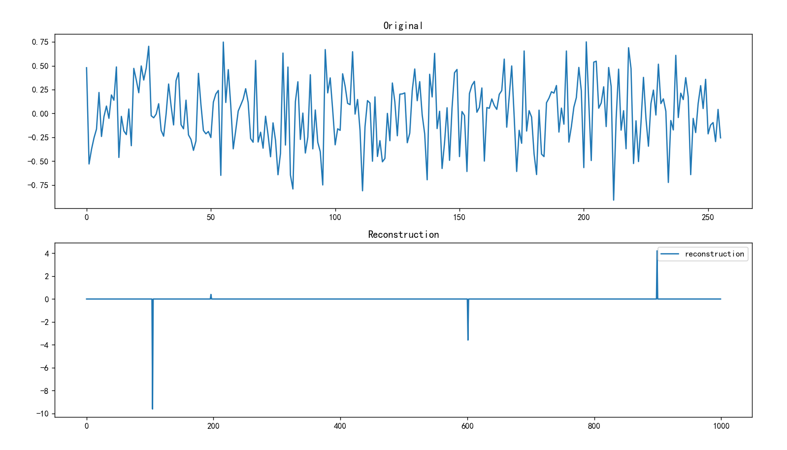
plt.subplot(2, 1, 1)
plt.plot(X[0])
plt.title("Original")
plt.subplot(2, 1, 2)
plt.plot(X_h.cpu().detach().numpy()[0], label="reconstruction")
plt.title("Reconstruction")
plt.legend()
plt.show()
|